Getting started with benchscofi
Introduction
The following section is an introduction to the functionalities of benchscofi. It is also available as interactive notebooks. In addition to the Python package stanscofi, which proposes standard procedures to train, and to validate drug repurposing classifiers, benchscofi implements several algorithms from the state-of-the-art and allows to assess their performance through adequate and quantitative metrics tailored to the problem of drug repurposing across a large set of publicly available drug repurposing datasets. It also implements algorithms for class density estimation, which permits the use of positive-unlabeled methods (see this post for an introduction to this type of algorithms).
Let’s create the folder containing the datasets:
$ mkdir -p datasets/
and import base librairies and off we go:
from stanscofi.utils import load_dataset
from stanscofi.datasets import Dataset
from stanscofi.training_testing import cv_training
from stanscofi.training_testing import weakly_correlated_split, random_simple_split
from stanscofi.validation import compute_metrics, plot_metrics, metrics_list
import stanscofi.validation
import numpy as np
import pandas as pd
import benchscofi
Note 1: As a general rule, functions are documented, so one can check out the inputs and outputs of a function func by typing:
help(func)
Note 2: To mesure your environmental impact when using this package (in terms of carbon emissions), please run the following command:
$ codecarbon init
to initialize the CodeCarbon config. For more information about using CodeCarbon, please refer to the official repository.
Benchmark pipeline
Let’s build a very simple pipeline for testing algorithms in benschcofi.
Parameters (and reproducibility)
Let’s fix the random seed and the decision threshold (to convert prediction scores to labels in {-1,0,+1}):
random_state = 1234
decision_threshold=0
Let’s select the dataset to run our pipeline on. We will consider the TRANSCRIPT dataset, which will be randomly split into a training dataset (80% of ratings) and a testing dataset (20% of ratings). If parameter split_randomly is set to False, the dataset will be split using the weakly_correlated approach, running a hierarchical clustering on drug features using the cosine metric:
dataset_names = ["TRANSCRIPT"]
split_params = {"metric": "cosine", "test_size": 0.2, "split_randomly": True}
We will store the parameters for each algorithm which is going to be tested in the following dictionary. Here, we will only consider the PMF algorithms (see in the next section all currently implemented algorithms):
algo_params = {
    "PMF": {
        'reg': 0.01,
        'learning_rate': 0.5,
        'n_iters': 160,
        'n_factors': 15,
        'batch_size': 100,
    },
}
Training and testing a single model on a single dataset
The following function splits the dataset in input, performs a 5-fold cross validation on the training set with the input algorithm, outputs predictions for the testing dataset, plots the validation figures and returns the validation metrics in a data frame:
nsplits=5
njobs=nsplits-1

def training_testing(
      dataset_name,       ## dataset name
      split_params,       ## split params
      algo,               ## algorithm name
      params,             ## algorithm params
      random_state,       ## seed
      decision_threshold, ## predictions
      k, beta ## for validation measures
    ):
    #############
    ## Dataset ##
    #############
    dataset_di = load_dataset(dataset_name, dataset_folder)
    dataset_di.setdefault("same_item_user_features", dataset_name=="TRANSCRIPT")
    dataset_di.setdefault("name", dataset_name)
    dataset = Dataset(**dataset_di)

    ############################
    ## Weakly correlated sets ##
    if (not split_params["split_randomly"]):
        (train_folds, test_folds), _ = weakly_correlated_split(
            dataset, split_params["test_size"], early_stop=1,
            metric=split_params["metric"], verbose=True
        )
    ######################
    ## Random splitting ##
    else:
        (train_folds, test_folds), _ = random_simple_split(dataset,
           split_params["test_size"], metric=split_params["metric"]
        )

    train_dataset = dataset.subset(train_folds, subset_name="Train_"+dataset_name)
    test_dataset = dataset.subset(test_folds, subset_name="Test_"+dataset_name)

    train_dataset.summary()
    test_dataset.summary()

    ###############
    ## Algorithm ##
    ###############
    __import__("benchscofi."+algo)
    model = eval("benchscofi."+algo+"."+algo)(algo_params[algo])

    ###############
    ## Training  ##
    ###############
    #model.fit(train_dataset, random_state)
    ######################
    ## Cross-validation ##
    results = cv_training(eval("benchscofi."+algo+"."+algo), params, train_dataset,
        threshold=decision_threshold, metric="AUC", k=k, beta=beta, njobs=njobs,
        nsplits=nsplits, random_state=random_state, show_plots=False, verbose=True,
        cv_type="random" if (split_params["split_randomly"]) else "weakly_correlated")
    model = results["models"][np.argmax(results["test_metric"])]

    #################
    ## Predictions ##
    #################
    scores = model.predict_proba(test_dataset)
    predictions = model.predict(scores, threshold=decision_threshold)

    model.print_scores(scores)
    model.print_classification(predictions)

    #################
    ## Validation  ##
    #################

    ## disease-wise metrics
    metrics, plot_args = compute_metrics(scores, predictions, test_dataset,
         metrics=metrics_list, k=k,beta=beta,verbose=1) ## run all metrics
    plot_args.update({"model_name": "PMF", "figsize": (8,8)})
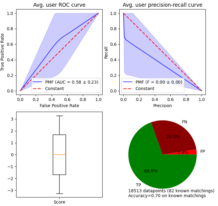
    plot_metrics(**plot_args)

    ## dataset-wide metrics
    y_test = (test_dataset.folds.toarray()*test_dataset.ratings.toarray()).ravel()
    y_test[y_test<1] = 0

    whole_metrics = [
            eval("stanscofi.validation."+metric)(y_test, scores.toarray().ravel(), k, beta)
            for metric in metrics_list if (metric not in ["Fscore", "TAU"])
    ]

    results = pd.concat(
      (
      pd.DataFrame(
            [whole_metrics],
            index=["Value"],
            columns=[m for m in metrics_list if (m not in ["Fscore","TAU"])]
            ).T,
       metrics
      ), axis=1)

    return results
Application of the pipeline
Let’s apply this pipeline on dataset TRANSCRIPT with algorithm PMF:
training_testing(
   dataset_names[0],
   split_params,
   [a for a in algo_params][0],
   algo_params[[a for a in algo_params][0]],
   random_state,
   decision_threshold,
   5, 1
)

Algorithms
Each algorithm algo with parameters contained in a dictionary params is accessible by the following code line:
model = benchscofi.algo.algo(params)
## which can be called using model.fit(...), model.predict(...)
The dictionary of default parameter values is available by typing:
model.default_parameters()
Contributions for new algorithms are open (see the README). Tags are associated with each method.
featurelessmeans that the algorithm does not leverage the input of drug/disease features.matrix_inputmeans that the algorithm considers as input a matrix of ratings (plus possibly matrices of drug/disease features), instead of considering as input (drug, disease) pairs.
PMF Probabilistic Matrix Factorization (using Bayesian Pairwise Ranking) implemented at this page. featureless matrix_input
PulearnWrapper Elkan and Noto’s classifier based on SVMs (package pulearn and paper). featureless
ALSWR Alternating Least Square Matrix Factorization algorithm implemented at this page. featureless
FastaiCollabWrapper Collaborative filtering approach collab_learner implemented by package fast.ai. featureless
SimplePULearning Customizable neural network architecture with positive-unlabeled risk.
SimpleBinaryClassifier Customizable neural network architecture for positive-negative learning.
NIMCGCN Jin Li, Sai Zhang, Tao Liu, Chenxi Ning, Zhuoxuan Zhang and Wei Zhou. Neural inductive matrix completion with graph convolutional networks for miRNA-disease association prediction. Bioinformatics, Volume 36, Issue 8, 15 April 2020, Pages 2538–2546. doi: 10.1093/bioinformatics/btz965. (implementation).
FFMWrapper Field-aware Factorization Machine (package pyFFM).
VariationalWrapper Vie, J. J., Rigaux, T., & Kashima, H. (2022, December). Variational Factorization Machines for Preference Elicitation in Large-Scale Recommender Systems. In 2022 IEEE International Conference on Big Data (Big Data) (pp. 5607-5614). IEEE. (pytorch implementation). featureless
DRRS Luo, H., Li, M., Wang, S., Liu, Q., Li, Y., & Wang, J. (2018). Computational drug repositioning using low-rank matrix approximation and randomized algorithms. Bioinformatics, 34(11), 1904-1912. (download). matrix_input
SCPMF Meng, Y., Jin, M., Tang, X., & Xu, J. (2021). Drug repositioning based on similarity constrained probabilistic matrix factorization: COVID-19 as a case study. Applied soft computing, 103, 107135. (implementation). matrix_input
BNNR Yang, M., Luo, H., Li, Y., & Wang, J. (2019). Drug repositioning based on bounded nuclear norm regularization. Bioinformatics, 35(14), i455-i463. (implementation). matrix_input
LRSSL Liang, X., Zhang, P., Yan, L., Fu, Y., Peng, F., Qu, L., … & Chen, Z. (2017). LRSSL: predict and interpret drug–disease associations based on data integration using sparse subspace learning. Bioinformatics, 33(8), 1187-1196. (implementation). matrix_input
MBiRW Luo, H., Wang, J., Li, M., Luo, J., Peng, X., Wu, F. X., & Pan, Y. (2016). Drug repositioning based on comprehensive similarity measures and bi-random walk algorithm. Bioinformatics, 32(17), 2664-2671. (implementation). matrix_input
LibMFWrapper W.-S. Chin, B.-W. Yuan, M.-Y. Yang, Y. Zhuang, Y.-C. Juan, and C.-J. Lin. LIBMF: A Library for Parallel Matrix Factorization in Shared-memory Systems. JMLR, 2015. (implementation). featureless
LogisticMF Johnson, C. C. (2014). Logistic matrix factorization for implicit feedback data. Advances in Neural Information Processing Systems, 27(78), 1-9. (implementation). featureless
PSGCN Sun, X., Wang, B., Zhang, J., & Li, M. (2022). Partner-Specific Drug Repositioning Approach Based on Graph Convolutional Network. IEEE Journal of Biomedical and Health Informatics, 26(11), 5757-5765. (implementation). featureless matrix_input
DDA_SKF Gao, C. Q., Zhou, Y. K., Xin, X. H., Min, H., & Du, P. F. (2022). DDA-SKF: Predicting Drug–Disease Associations Using Similarity Kernel Fusion. Frontiers in Pharmacology, 12, 784171. (implementation). matrix_input
HAN GWang, Xiao, et al. “Heterogeneous graph attention network.” The world wide web conference. 2019. (implementation).
PUextraTrees Wilton, Jonathan, et al. “Positive-Unlabeled Learning using Random Forests via Recursive Greedy Risk Minimization.” Advances in Neural Information Processing Systems 35 (2022): 24060-24071. (implementation).
XGBoost Chen, Tianqi, and Carlos Guestrin. “Xgboost: A scalable tree boosting system.” Proceedings of the 22nd acm sigkdd international conference on knowledge discovery and data mining. 2016. (implementation).
Row-wise performance metrics
An additional performance measure has been added compared to stanscofi.
Negative Sampling AUC (NS-AUC)
The row-wise (ie, disease-wise) AUC score comes from this paper and allows to quantify how much the initial order of drug-disease pairs (as given by the true labels t) is preserved in the ranking induced by the prediction scores p.
If \(\Omega^{*}_\text{di}(t) \triangleq \{\text{drug} \mid t[\text{drug},\text{di}] = *\}\), compute for each disease di the following score, which is the average number of times a positive pair (+1) is scored higher than a negative (-1) or unknown (0) pair:
Finally, the averaged NS-AUC score is:
In code:
from benchscofi.utils.rowwise_metrics import calc_auc
calc_auc(scores, dataset, transpose=False)
When transpose is set to True, the score is computed drug-wise instead of disease-wise.
Class density estimation methods
Cost-sensitive approaches and positive-unlabeled learning (see this post for an introduction to this type of algorithms) crucially rely on the knowledge of outcome prior \(\pi\), which might have a large impact on the quality of the recommendations. \(y \in \{−1, 0, 1\}\) are the accessible labels. Let us denote \(s \in \{−1, 1\}\) the true labels, and \(v\) is the feature vector. Under the usual assumptions made in Positive-Unlabeled (PU) learning:
benchscofi provides implementations of several class prior estimation methods, shown below. We will test their performance on randomly generated datasets:
import stanscofi.datasets
import stanscofi.utils
import stanscofi.training_testing
import numpy as np
import pandas as pd

import benchscofi
import benchscofi.utils
from benchscofi.utils import prior_estimation
Assumptions on datasets
As well as the drug repurposing dataset TRANSCRIPT, we will also consider synthetic datasets where the true value \(\pi\) is known in advance, so as to test the class density estimation approaches. The following functions prints naive estimators and the true values (when available) of datasets:
def print_naive_estimators(dataset, labels_mat, true_args):
    pos, neg = np.sum(dataset.ratings.data>0), np.sum(dataset.ratings.data<0)
    known, total = np.sum(dataset.ratings.data!=0), np.prod(dataset.ratings.shape)
    pos_known = pos/known
    pos_total = pos/total
    known_total = known/total
    pos_unk = pos/(total-known)
    neg_pos = neg/pos
    if (labels_mat is None): ## no access to true values
        pos_known_true = np.nan
    else:
        pos_known_true = np.sum(labels_mat.values>0)/np.prod(labels_mat.values.shape)
    return pd.DataFrame(
        [
            [true_args[arg] for arg in true_args]
            +[pos_known, known_total, pos_unk, pos_known_true,
              pos_total/true_args["pi"] if ("pi" in true_args) else np.nan,
              pos_total/pos_known_true if (labels_mat is not None) else np.nan,
              neg_pos]
        ],
        columns=[arg for arg in true_args]+[
                "#Pos/#Known",               ## ratio b/w positive and accessible pairs
                "#Known/#Total~sparsity",    ## ratio b/w known and 1-sparsity number
                "#Pos/#Unk",                 ## ratio b/w positive and unknown pairs
                "#Pos/#Known(true)~pi",      ## ratio b/w positive and all pairs
                "#Pos/(#Total*pi)~c",
                "(#Pos/#Total)/(#Pos/#Known(true))~c",
                "#Neg/#Pos"],
        index=["Value"],
    )
We will generate several synthetic datasets with \(10,000\) datapoints, \(100\) features, with the same random seed:
synthetic_params = {
    "N":10000, "nfeatures":100, "mean":2, "std":0.1, "exact": True, "random_state": 1234,
}
Censoring setting
Assume that \(s \in \{-1,1\}\) are the true labels, \(y \in \{0,1\}\) are the accessible labels (note that accessible negative samples are missing), and \(v \in \mathbb{R}^d\) are the feature vectors. Samples \((v,s) \sim p(v,s)\), and then are made accessible as follows \(y \sim p(\cdot \mid v, s=1)\) and \(\mathbb{P}(y \neq 0 \mid v, s=-1) = p(y=-1 \mid v, s=1) = 0\). This setting relies on the SCAR assumption [ref]:
Note that
[ref] Elkan, Charles, and Keith Noto. “Learning classifiers from only positive and unlabeled data.” Proceedings of the 14th ACM SIGKDD international conference on Knowledge discovery and data mining. 2008.
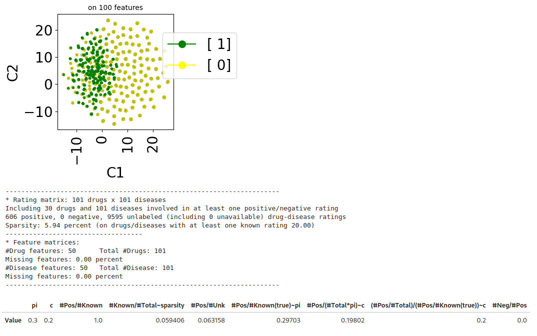
The following lines generate a synthetic dataset which matches the specifications of the censoring setting. In that setting, there are only positive (\(y=1\)) and unlabeled (\(y=0\)) samples (i.e., all negative samples are unlabeled).
from benchscofi.utils.prior_estimation import generate_Censoring_dataset

true_args_censoring = {"pi": 0.3, "c":0.2}
censoring_params = {}
censoring_params.update(true_args_censoring)
censoring_params.update(synthetic_params)

censoring_di, censoring_labels_mat = generate_Censoring_dataset(**censoring_params)
censoring_dt = stanscofi.datasets.Dataset(**censoring_di)
censoring_dt.visualize(withzeros=True, figsize=(3,3), dimred_args={"n_neighbors": 10})

censoring_dt.summary()

print_naive_estimators(censoring_dt, censoring_labels_mat, true_args_censoring)
## pi ~ #pos/#total in the true labels matrix which is OK
## c ~ (#pos/#total)/pi in the ratings matrix which is OK

Case-Control setting
Assume that \(s \in \{-1,1\}\) are the true labels, \(y \in \{-1,0,1\}\) are the accessible labels, and \(v \in \mathbb{R}^d\) are the feature vectors. Positive pairs \(v \sim p_+ = p(\cdot | y=+1)$\), negative pairs \(v \sim p_- = p(\cdot | y=-1)\), and unlabeled pairs \(v \sim p_u = \pi p_+ + (1-\pi)p_-\) (where \(\pi := \mathbb{P}(s = 1) \in (0,1)\) is the class-prior probability). This setting relies on the Invariance of Order assumption [ref]:
[ref] Kato, Masahiro, Takeshi Teshima, and Junya Honda. “Learning from positive and unlabeled data with a selection bias.” International conference on learning representations. 2018.
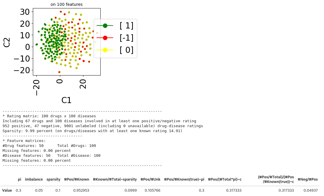
Generating a case-control dataset:
from benchscofi.utils.prior_estimation import generate_CaseControl_dataset

true_args_casecontrol = {"pi": 0.3, "imbalance": 0.05, "sparsity": 0.1}
casecontrol_params = {}
casecontrol_params.update(true_args_casecontrol)
casecontrol_params.update(synthetic_params)

casecontrol_di, casecontrol_labels_mat = generate_CaseControl_dataset(**casecontrol_params)
casecontrol_di.update({"name": "casecontrol"})
casecontrol_dt = stanscofi.datasets.Dataset(**casecontrol_di)
casecontrol_dt.visualize(withzeros=True, figsize=(3,3), dimred_args={"n_neighbors": 10})

casecontrol_dt.summary()

print_naive_estimators(casecontrol_dt, casecontrol_labels_mat, true_args_casecontrol)
## pi ~ #pos/#total in the true labels matrix which is OK
## sparsity ~ #known/#total in the ratings matrix which is OK

Methods relying on a pretrained classifier
Training a classifier
We also generate a validation dataset which is produced in the same fashion as the training dataset. We first consider the synthetic Censoring dataset.
(traintest_folds, val_folds), _ = stanscofi.training_testing.random_simple_split(censoring_dt,
      0.2, metric="euclidean")
traintest_dataset = censoring_dt.subset(traintest_folds, subset_name="Train Test")
val_dataset = censoring_dt.subset(val_folds, subset_name="Validation")
We train a Positive-Unlabeled classifier called PUlearn [ref] on the training subset, and keep the validation subset to compute estimators of the class prior.
[ref] Charles Elkan and Keith Noto. Learning classifiers from only positive and unlabeled data. In Proceedings of the 14th ACM SIGKDD international conference on Knowledge discovery and data mining, pages 213–220, 2008.
from benchscofi.PulearnWrapper import PulearnWrapper

results = stanscofi.training_testing.cv_training(PulearnWrapper, None, traintest_dataset,
      threshold=0, metric="AUC", k=5, beta=1, njobs=1, nsplits=5, random_state=rseed,
      cv_type="random", show_plots=False, verbose=True)
Estimators for Censoring datasets
In the censoring setting: Three estimators \(e_1\), \(e_2\) and \(e_3\) of \(c := \mathbb{P}(s=1 \mid y \neq 0)\) proposed by [ref]. Given a trained classifier \(\widehat{\theta}\), and a validation set \(\mathcal{V} := \{ (v,y) \mid y \in \{-1,0,1\}, v \in \mathbb{R}^d \}\),
If \(f_{\widehat{\theta}}(v)=\mathbb{P}(s=1 | v)\) for any \(v\), then \(e_1=c\). It is assumed that \(e_3 \leq c\). Authors recommend using \(e_1\). But that approach requires having access to a supplementary validation dataset with labelled samples. One can retrieve an approximation of \(\pi:=\mathbb{P}(s=1)\) by using \(c\pi = \mathbb{P}(y=1) \approx \sum_{(v',+1) \in \mathcal{V}} (f_{\widehat{\theta}}(v'))_+\)
[ref] Charles Elkan and Keith Noto. Learning classifiers from only positive and unlabeled data. In Proceedings of the 14th ACM SIGKDD international conference on Knowledge discovery and data mining, pages 213–220, 2008. Assume that there are no unlabeled (all 0’s are negative). Then we expect the estimators to determine that $c=1$, as no unlabeled are assumed.
trained_classifier = results["models"][np.argmax(aucs_whole)]
scores_test = m.predict_proba(val_dataset).toarray().ravel()
y_test = (val_dataset.folds.toarray()*val_dataset.ratings.toarray()).ravel()
y_test_ = y_test.copy()
pred_scores = np.array([max(min(s,1),0) for s in scores_test])

[e1,pi1], [e2,pi2], [e3,pi3] = [
   prior_estimation.data_aided_estimation(pred_scores, y_test_, estimator_type=i)
   for i in [1,2,3]
]

pd.DataFrame(
   [
       [e1, e2, e3, pi1, pi2, pi3],
       [true_args_censoring["c"]]*3+[true_args_censoring["pi"]]*3,
   ]
, index=["Estimated", "True"], columns=["e1", "e2", "e3", "pi1", "pi2", "pi3"])

Bayes regret approach for Case-Control datasets
In the case-control setting: [ref1, Theorem 4] shows that if the supports for \(p_+\) and \(p_-\) are different
The issue is that the equation shown above can’t be computed exactly in practice. As mentioned in [ref2], a possible approach to approximate \(\hat{\pi}\) is to regress a specific model (given in [ref2]) on the points of the corresponding ROC curve, and use the fitted model to extract the slope at the right-hand side of the curve, which is \(\hat{\pi}\).
[ref1] Scott, Clayton, and Gilles Blanchard. “Novelty detection: Unlabeled data definitely help.” Artificial intelligence and statistics. PMLR, 2009.
[ref2] Sanderson, Tyler, and Clayton Scott. “Class proportion estimation with application to multiclass anomaly rejection.” Artificial Intelligence and Statistics. PMLR, 2014.
(traintest_folds, val_folds), _ = stanscofi.training_testing.random_simple_split(
    casecontrol_dt, 0.2, metric="euclidean")
traintest_dataset = casecontrol_dt.subset(traintest_folds, subset_name="Train Test")
val_dataset = casecontrol_dt.subset(val_folds, subset_name="Validation")

print("Training/testing set")
traintest_dataset.summary()
print("Validation set")
val_dataset.summary()

results = stanscofi.training_testing.cv_training(PulearnWrapper, None,
     traintest_dataset, threshold=0, metric="AUC", k=5, beta=1, njobs=1,
     nsplits=5, random_state=rseed, cv_type="random", show_plots=False,
     verbose=True)

pi_star1, pi_star2 = [
   prior_estimation.roc_aided_estimation(scores_test, y_test, regression_type=i, verbose=True,
                                         show_plot=(i<2)) for i in [1,2]
]

pd.DataFrame(
   [
       [pi_star1, pi_star2],
       [true_args_censoring["pi"]]*2,
   ]
, index=["Estimated", "True"], columns=["pi*1", "pi*2"])

Penalized divergences for Case-Control datasets
Contrary to the last two approaches, these methods do not use a pretrained classifier. \(\lambda\) and \(\sigma\) are regularization parameters, and \(p\) (resp., \(u\)) is the total number of positive (resp., unlabeled) samples).
L1-penalized divergence
Using L1-distance penalized divergence [ref] amounts to minimizing the following scalar function:
[ref] Christoffel, Marthinus, Gang Niu, and Masashi Sugiyama. “Class-prior estimation for learning from positive and unlabeled data.” Asian Conference on Machine Learning. PMLR, 2016.
Pearson-penalized divergence
Using the Pearson penalized divergence [ref] amounts to minimizing the following scalar function:
\(\text{ and } H := \left[\frac{1}{u}\sum_{j \leq u}\left(\mathcal{N}(x_l, \sigma^2 \text{Id})(x_j)\right)_{0 \leq l \leq u+p}, \frac{1}{p}\sum_{i \leq p}\left(\mathcal{N}(x_l, \sigma^2 \text{Id})(x_i)\right)_{0 \leq l \leq u+p} \right] \in \mathbb{R}^{(u+p+1) \times 2} \;,\)
\(R := \left[^{0}_{(0)_{(u+p) \times 1}} ,^{(0)_{1 \times (u+p)}}_{Id_{(u+p) \times (u+p)}}\right] \in \mathbb{R}^{(u+p+1) \times (u+p+1)} \;,\)
\(G := \frac{1}{u+p} \sum_{i \leq u+p} \left(\mathcal{N}(x_l, \sigma^2 \text{Id})(x_i)\right)_{0 \leq l \leq u+p}^\top\left(\mathcal{N}(x_l, \sigma^2 \text{Id})(x_i)\right)_{0 \leq l \leq u+p} \in \mathbb{R}^{(u+p+1) \times (u+p+1)}\)
\(\text{where } \forall x \ , \ \mathcal{N}(x_0, \sigma^2 \text{Id})(x)=1\).
[ref] Du Plessis, Marthinus Christoffel, and Masashi Sugiyama. “Semi-supervised learning of class balance under class-prior change by distribution matching.” Neural Networks 50 (2014): 110-119.
Tests
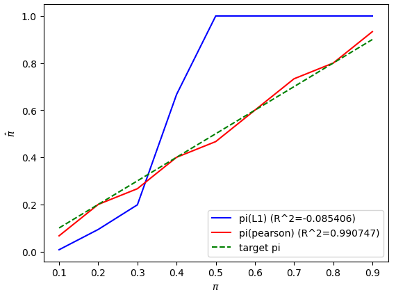
Let’s now compare the different penalized divergence-based approaches:
import matplotlib.pyplot as plt
from sklearn.metrics import r2_score

from benchscofi.utils import prior_estimation

## One could also have more precise estimates by iterating on several random seeds
def test_estimator(pi_true):
   pi_hats, pi_hats2 = [], []
   for i, pi_t in enumerate(pi_true):
       true_args_casecontrol = {"pi": pi_t, "imbalance": 0.0001, "sparsity": 0.9999}
       casecontrol_params = {}
       casecontrol_params.update(true_args_casecontrol)
       casecontrol_params.update(synthetic_params)
       casecontrol_params.update({"N": 250})
       casecontrol_di, _ = generate_CaseControl_dataset(**casecontrol_params)
       casecontrol_dt_pi = stanscofi.datasets.Dataset(**casecontrol_di)
       X, y, _, _ = stanscofi.preprocessing.meanimputation_standardize(casecontrol_dt_pi)
       pi_hat = prior_estimation.divergence_aided_estimation(X, y, lmb=1., sigma=.01,
             divergence_type="L1-distance")
       pi_hat2 = prior_estimation.divergence_aided_estimation(X, y, lmb=1., sigma=.01,
             divergence_type="Pearson")
       pi_hats.append(pi_hat)
       pi_hats2.append(pi_hat2)
       print("Test %d, pi=%f, pi(L1)=%f pi(pearson)=%f" % (i+1, pi_t, pi_hat, pi_hat2))
   R = r2_score(pi_true, pi_hats)
   plt.plot(pi_true, pi_hats, "b-", label="pi(L1) (R^2=%f)" % R)
   R2 = r2_score(pi_true, pi_hats2)
   plt.plot(pi_true, pi_hats2, "r-", label="pi(pearson) (R^2=%f)" % R2)
   plt.plot(pi_true, pi_true, "g--", label="target pi")
   plt.xlabel(r"$\pi$")
   plt.ylabel(r"$\hat{\pi}$")
   plt.legend()
   plt.show()

test_estimator([0.1,0.2,0.3,0.4,0.5,0.6,0.7,0.8,0.9])
