Introduction to PU learning

Drug repurposing is a paradigm for drug development, where drug discovery focuses on already commercialized molecules. The key idea is that if those molecules are considered, turning them into appropriate and safe drugs for patients is much faster. As described in a previous post, to perform drug repurposing, one has access to reported outcomes of past clinical trials, with possibly additional information about drugs and diseases. Reported effects can be positive (i.e., the corresponding clinical trial has successfully concluded that the drug might treat the pathology at study) or negative (the clinical trial has failed due to lack of efficacy or reported toxicity effects).

Most of the time, compared to the total number of possible drug-disease matchings, the number of known outcomes is usually dramatically lower. Moreover, the number of known matchings is too small to train a classical binary classifier, such as logistic regression or a Support Vector Machine (SVM). One might argue that to overcome this lack of data, it suffices to consider all unknown outcomes as negative (or, less intuitively, perhaps, positive). However, the information that a given clinical trial has not been performed is different than assuming that a drug-disease matching is negative and might induce considerable bias in our underlying model.

The problem of learning a classification model in circumstances where some of the data is not annotated arises as well in advertising and recommender systems (e.g., in movie/series recommendations on your favorite streaming service!), To leverage this implicit information (also called feedback), several papers have already proposed using with collaborative filtering, and more specifically, positive-unlabeled (PU) learning [1].

Illustration with a neural network

For example, we will implement a neural network model that considers unlabeled data in its loss. A neural network is a nested function of many parameters (often alterning between linear and non-linear terms) which takes as input a feature vector corresponding to a data point, and outputs (in our case) a score between 0 and 1. That score corresponds to the probability $P(y=1 \mid x)$ for a sample with feature vector $x$ of being positive: 0 for an outcome labeled negative with high confidence, and 1 for an outcome labeled positive with high confidence. Neural networks are extremely versatile models, which are able to mimic a large variety of mathematical functions.

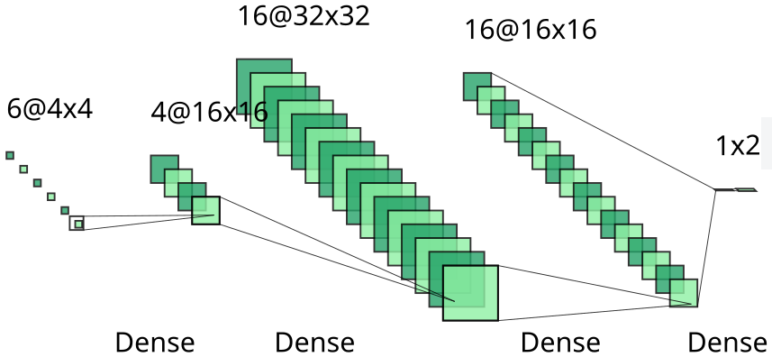
In order to assess the power of positive-unlabeled learning over classical binary learning, we will consider the same (very small) architecture for both models, with 4 hidden dense layers of dimensions 4, 16, 32, and 16 alternating with ReLU activation functions. That neural network is represented below. In our example, feature vectors are of length 6, and the network outputs a score for each possible class (positive or negative).

The next two sections will be a bit mathematical. If you only care about the result, please directly go to the Results part.

Architecture of our neural network in binary and PU classification.

A simple binary classifier

Training the neural network on our data means in practice optimizing all parameters of the network such that these parameters optimize (maximizing or minimizing) a given function, called loss when it should be minimized. The idea is that optimizing for this loss should make our model performant for downsteam tasks (for instance, drug repurposing). In practice, to ease the derivations, we assume that the neural network computes a value akin to a logit, that is, we obtain at the exit of the last layer

\[L(x) := \log(P(y=1\mid x)/(1-P(y=1 \mid x))),\]

where $x$ is the feature vector and $y$ is the variable associated with the outcome class, and outputs as a score $(1+\exp(-L(x)))^{-1}$ between 0 and 1 (that is, the sigmoid function applied to the logit value).

When considering the binary data, that is, assuming that unlabeled datapoints are actually negative, a popular loss function is the binary cross-entropy function, also called log loss. The underlying idea behind log loss is that, for a binary classification, if we assume that the score outputted by the neural network correspond to the probability of the input datapoint to be positive, then we want to maximize the score for known positive points, and to minimize the score for known negative points. For a more detailed (and mathematical) explanation on log loss, please refer to this very nice post.

Assume that there are $n$ datapoints of the form $(x,y)$, where $x$ is the feature vector of length 6 and $y$ the outcome class (0: negative or unlabeled, 1: positive). $n=n_P + n_U$, where $n_P$ is the number of positive samples, and $n_U$ is the number of unlabeled or negative samples. Considering the set of parameters $\theta$ and

\[F_\theta := (1+\exp(-L_\theta(x)))^{-1}\]

the function encoded by our neural network with parameters $\theta$, let us write down the expression of the empirical log loss on our dataset,

\[H(\theta) := -\frac{1}{n_P} \sum_{(x,y),y=1} y \log F_\theta(x) -\frac{1}{n_U} \sum_{(x,y),y=0} (1-y) \log(1-F_\theta(x)) .\]

Assume that our model assigns 1 to every positive datapoint, and 0 to every negative datapoint. Replacing the $F_\theta(x)$ with the appropriate values, it is easy to see that $H(\theta)=0$ in that case, meaning indeed that our model is perfect.

A simple PU classifier

Now, if we consider unlabeled datapoints to be a mixture of positive and negative samples, we can no longer use the previous loss function with our full dataset. In particular, we make the assumption that actually, an unlabeled datapoint is $100\pi\%$ of the time a positive datapoint and thus $100(1-\pi)\%$ a negative one, where $\pi$ is an unknown value between 0 and 1. Case $\pi=0$ is the binary classification mentioned above. Formally, it means that, considering -1 as the class of negative samples

\[P(y=0 | x) = \pi P(y=1 | x) + (1-\pi) P(y=-1 | x).\]

In that context, assume that there are $n$ datapoints of the form $(x,y)$, where $x$ is the feature vector of length 6 and $y$ the outcome class (0: negative or unlabeled, 1: positive). $n=n_P + n_U$, where $n_P$ is the number of positive samples, and $n_U$ is the number of unlabeled or negative samples. We have to rewrite the log loss above. Using our assumption, we get that

\[P(y=-1 | x) = \frac{1}{1-\pi}P(y=0 | x) - \frac{\pi}{1-\pi}P(y=1 | x).\]

Replacing that in the previous empirical (binary) log loss expression and refactoring, by taking advantage of our logit assumption $F_\theta := (1+\exp(-L_\theta(x)))^{-1}$, yields the following expression

\[H(\theta) := \frac{2\pi - 1}{n_P(\pi - 1)} \sum_{(x,y),y=1} (T_\theta(x) - L_\theta(x)) - \frac{1}{n_U(1 - \pi)}\sum_{(x,y),y=0} T_\theta(x),\]

where $T_\theta(x):=\log \exp(L_\theta(x) + 1)$.

Implementation in Python

In order to implement the binary and PU classifiers described above, we use models SimplePULearning and SimpleBinaryClassifier in the benchscofi Python package (described in a previous post). We also share the associated Python file.

Results

Principal Component Analysis (PCA) plots for our binary classifier (left) and PU classifier (right), in a synthetic dataset with 200 positive datapoints and 100 negative datapoints, on 300 drugs and 300 diseases. For each plot, the blob on the left-hand side is the set of positive datapoints, and the right one is the set of negative datapoints. The color (red for negative and green for positive) corresponds to the labels given by the neural network.

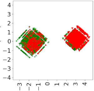
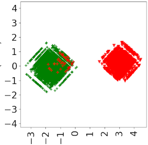
We can observe that, compared to the PU classifier, the classical binary approach greatly overestimates the number of negative samples (indeed, since it considers that all samples but positive ones are negative).

Notes

Note that all the post still holds if the length of your feature vectors is different from 6 ;)

There is a large variety of PU learning algorithms and assumptions on unlabeled data, each producing different types of models, so feel free to check out the review in References. Some of them are implemented in our package benchscofi.

One might wonder how to find the appropriate value of $\pi$ in our PU model. This problem has been investigated in the literature, yielding several methods to estimate the appropriate value of $\pi$. Some of them are also implemented in benchscofi. In order to see how to use those methods, and how they perform in a synthetic setting, please refer to the corresponding Jupyter notebook.

References

[1] Bekker, Jessa, and Jesse Davis. “Learning from positive and unlabeled data: A survey.” Machine Learning 109 (2020): 719-760.

Neural network architecture image was generated using NN-SVG.