Introduction to pathway enrichment (II)

This post is the second part of this one. We will use the same running example on epileptic mice exposed to a CSF1R inhibitor. In the previous post, one approach for pathway enrichment, named OverRepresentation Analysis (ORA), has been described. But remember that this method required to “arbitrarily” identify a list of genes of interest (possibly by a cutoff) and to separate the analysis of up-regulated and down-regulated genes. We now introduce Gene Set Enrichment Analysis [1] which will tackle both issues. Again, we will rely on WebGestalt [2] to run GSEA on the mouse data.

But anyway, let’s cut to the chase: what is GSEA?

2. Gene Set Enrichment Analysis (GSEA)

As in the previous blog post, assume that we have a list of ranked genes, ordered by their decreasing score, and a pathway P that contains several genes. Are genes in P randomly distributed in the ranking, or are they primarily at the top or at the bottom of the ranking?

2.1 Definition

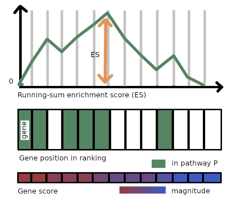
An enrichment score for P is computed by walking down the gene ranking $s_1 \geq s_2 \geq \dots \geq s_N$ (ordered by decreasing score). At the position $i$ of the ranking, we augment a counter if the gene at position $i$ belongs to P: we decrease it otherwise. The augmenting step depends on the magnitude of the score. Then we take the maximum value reached by that counter at any position in the ranking as the enrichment score. That value is higher if the distribution of genes from the pathway in the ranking is non-random.

More formally, we define the enrichment counter ES in the ranking of $N$ genes for the pathway P. We denote the sum of scores in absolute value associated with all the genes in both the ranking and P

\[S_P = \sum_{g \in P} |s(g)|\;.\]

Then, if the gene $g_1$ is at position $1$ with the score $s_1$ in the ranking

\[\text{ES}[0] = \begin{cases} \frac{|s_1|}{S_P} & \text{ if $g_1$ belongs to P} \\ -\frac{1}{N-|P|}& \text{ otherwise} \end{cases}\;.\]

Let’s go to position $2$ with score $s_2$ and gene $g_2$. Again

\[\text{ES}[1] = ES[0] + \begin{cases} \frac{|s_2|}{S_P} & \text{ if $g_2$ belongs to P} \\ -\frac{1}{N-|P|}& \text{ otherwise} \end{cases}\;.\]

We proceed iteratively over the ranking until we get the following value at the last position $N$

\[\text{ES}[N] = ES[N-1] + \begin{cases} \frac{|s_N|}{S_P} & \text{ if $g_N$ belongs to P} \\ -\frac{1}{N-|P|}& \text{ otherwise} \end{cases}\] \[= \underbrace{\sum_{j \leq N, g_j \in P} \frac{|s_j|}{S_P}}_\text{the "weighted" distribution of hits for P} - \underbrace{\sum_{j \leq N, g_j \notin P} \frac{1}{N-|P|}}_\text{the random distribution for genes not in P}\;.\]

The enrichment score is then

\[ES(P) = \max_{i \leq N} \text{ES}[i]\;,\]

which is represented by a vertical arrow in the figure above. Now we obtained a statistic that quantifies the deviation of the distribution of hits for P (that is, genes from P also present in the ranking) from a random distribution. But it is not enough to ensure that that enrichment is significant, even if the resulting score is very large. For instance, imagine a (dummy and extreme) case where all scores for genes are actually the same. Then we could possibly use any order on the genes, for example, the one where all genes in P are at the top. In that case, the enrichment score would be very high, but it is clear that such an enrichment does not really hold. Then we need to compute how much chance contributes to the actual enrichment score.

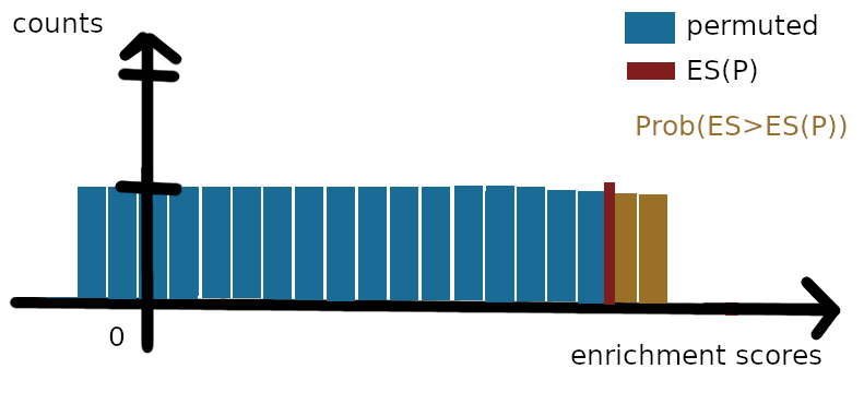
To do so, we can compute an “empirical” probability (p-value) of change contributing to the enrichment score using a number $n_p$ of permutations. For instance, we reorder randomly the genes in the ranking while keeping the same decreasing order on the scores, such that genes are often assigned to different score than initially$^1$. For each of these $n_p$ permutations of the genes, we compute again the enrichment score, since genes in the pathway are most likely not at the same position as before the permutation. Once we have the $n_P=1,000;10,000;…$ enrichment scores from permutations and the initial ES(P), we can compute a nominal p-value corresponding to the estimated probability of the enrichment score being larger than the computed value ES(P), corresponding to the area in yellow in the figure below. If that probability is large, probably most of the contribution to the score ES(P) comes from chance, as many different permutations allow to reach that value. So we are looking for pathways for which the probability of obtaining any larger enrichment value by simple permutation is low.

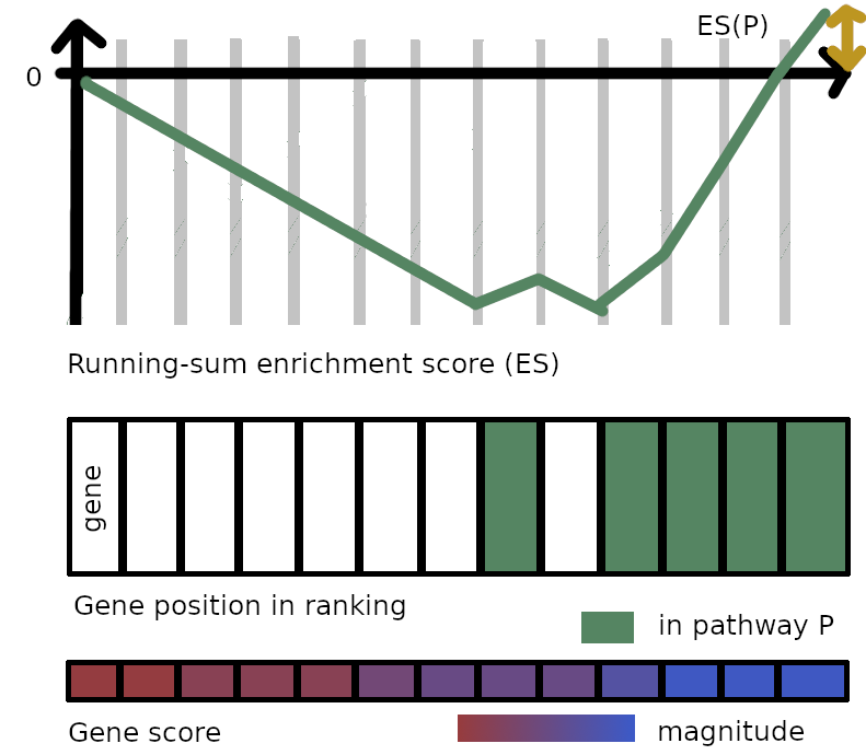
Finally, GSEA computes the z-score of the enrichment score for the pathway, called the normalized enrichment score (NES), that is, ES(P) divided by the mean enrichment score across permutations, and corrects the p-value across gene sets to get a false discovery rate (FDR) similarly to ORA. Intuitively, the NES for pathway P is (1) positive and large ($\gg 1.5$) when there are many genes from P at the top of the ranking, and conversely, (2) negative and large ($\ll -1.5$) when many genes from P are present at the bottom of the ranking. Why (1) is true is probably obvious. As for (2), it suffices to notice the symmetry with the first figure of the post.

2.2 Running a GSEA with WebGestalt

From the table that we have downloaded last time from GEO2R, we create a file with the extension .rnk with two columns, the gene identifier and the score, and remove the column titles, and sort genes by descending score value. Contrary to ORA, we provide the score for all measured genes, and not only significantly up- or down-regulated genes. We actually combine in one single file the list of genes of interest and the background list.

Once on WebGestalt, we select the species (Mus musculus), the gene annotations (Functional database > geneontology, Biological Process NoRedundant), and upload the .rnk file with the proper identifier type. At that point, you should see the following page

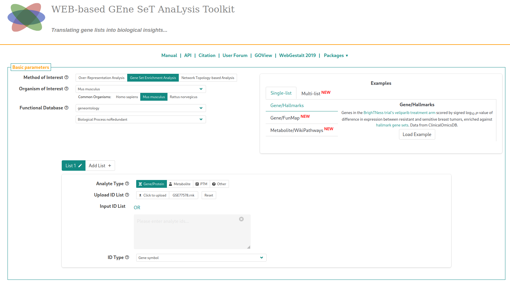
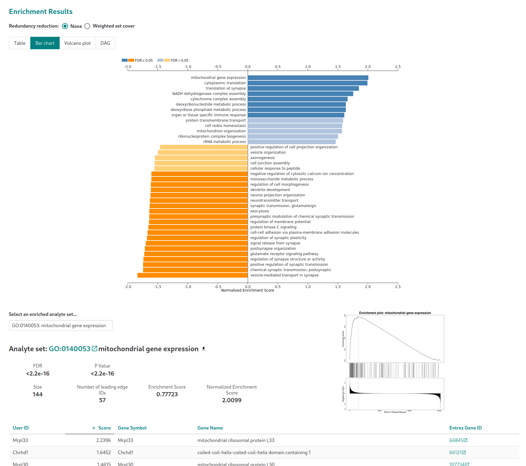
In the “Advanced parameters” tab, similarly to what was suggested for the ORA analysis, choose to display enriched pathways with FDR lower than 20% (“Significance level”) instead of the top enriched pathways. The analysis is started by clickling on the “Submit” button. Another parameter to change, contrary to ORA, is the number of permutations. Set it to 10,000. Running the analysis with the default parameters (after a short waiting time) will$^{2}$ lead to this page

2.3 Common pitfalls in GSEA

Number of permutations

In ORA, the measure of the significance of the enrichment (p-value) is directly derived from the hypergeometric test which quantifies the probability of having k hits in a list among a pathway. Here, GSEA only builds a$^{3}$ statistic related to the hits and then produces an empirical p-value based on multiple random permutations. On the one hand, the more permutations we run, the most accurate the p-value that we compute$^{4}$. On the other hand, those computations are time-expensive.

As a general rule, people use $n_P=1,000$ (eg. in the GSEA paper), but we would rather suggest $n_P=10,000$ and to rerun at least once other $10,000$ permutations to see if there is any enrichments that is missing (and then, that should be ignored for interpretation).

Overlap between pathways

Like in ORA, the p-values are not corrected for genes belonging to several pathways at a time. We suggest using the “non redundant” versions of pathways.

Identification of enriched pathways

Similarly to what was said for ORA, it is generally a bad idea to take into account non significantly enriched pathways (say, FDR>20%).

Comparison between ORA and GSEA

We compare the bar plots with enrichment scores (ORA, on the left) and normalized enrichment scores (GSEA, on the right) obtained on the epileptic mice data set.

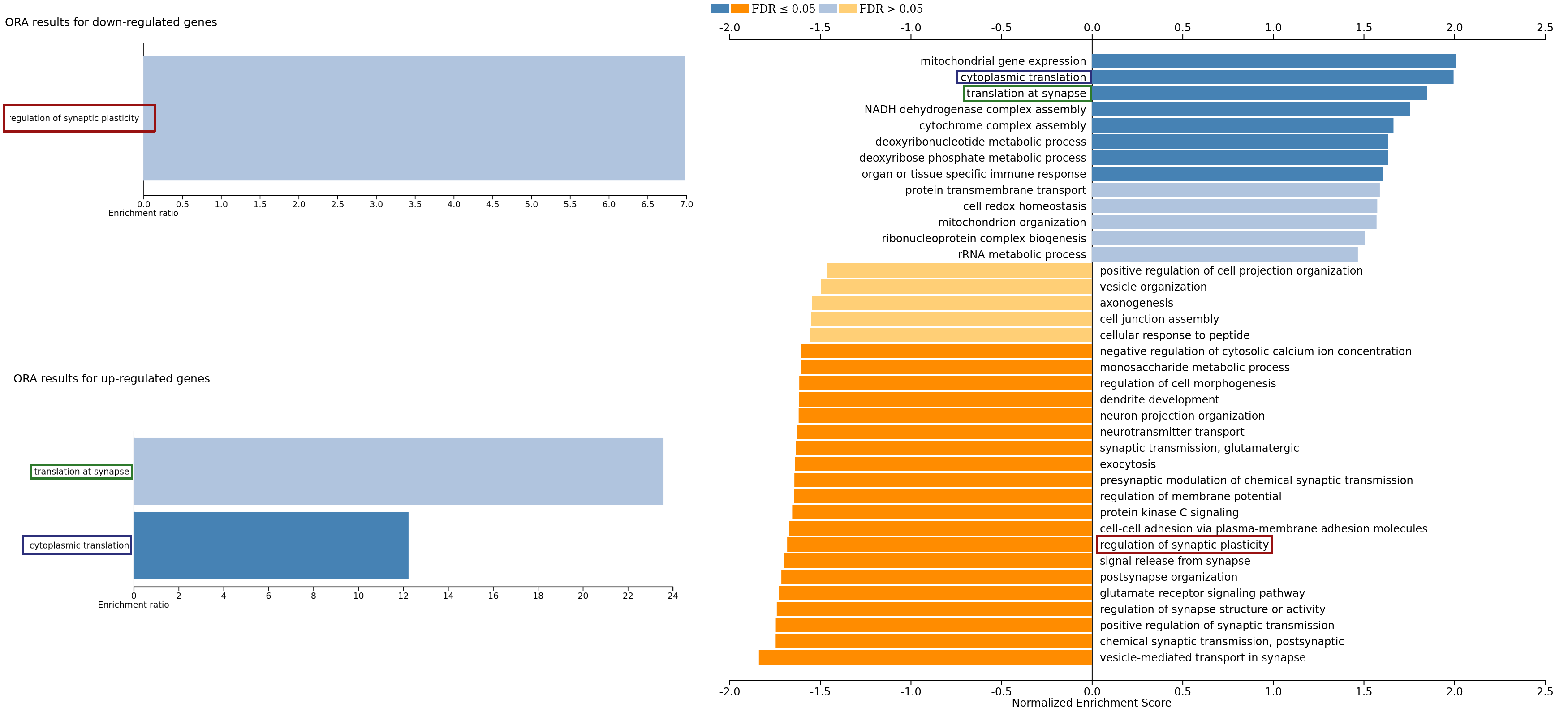
In a data set with a larger enough number of samples such as that one, we can recover by GSEA (sometimes with larger significance) the enrichments in ORA, both for up-regulated and down-regulated genes. This is probably to the fact that the threshold on the score for ORA yields a low number of genes ($\approx 60$) which is often not enough for statistical power. However, giving too many genes as input to ORA might bias the analysis, as it would perhaps include not significantly changing genes.

Conclusion

Most of the time, GSEA is favored over ORA when access to valid genes scores is available (for instance, the $-\log_{10}(\text{adj-p}) \times \log_2(\text{FoldChange})$). However, if only a list of a few hundred genes is available without any score, then ORA is probably best. Note that there are other types of enrichment analyses that we did not mention, but we encourage you to check them out. This post concludes our flash lecture on pathway enrichment. As it was meant to be an introduction, we did not dwell much on the most mathematical aspects of these analysis, in particular, the statistical correction for the number of genes in a pathway and for the number of pathways. Feel free to send feedback on our $\mathbb{X}$/Twitter or on the contact page!

Next time, we will talk about the results of our large-scale benchmark on collaborative filtering for drug repurposing. Stay tuned!

Footnotes

$^{1}$ This is not exactly the permutation model in the original GSEA paper, as they assume access to the samples on which the score per gene is computed. Here, since we only assume that we have access to the scores themselves, we use a different permutation model which can be implemented in practice.

$^{2}$ Probably, as the number of permutations is quite large. However, there is a part of non determinism in that case, especially with the online version of WebGestalt. With a script, you might be able to generate fully reproducible analyses.

$^{3}$ It is actually a “Kolmogorov-Smirnov statistic”, weighted by the score of each gene (because we consider the case $p=1$ in the GSEA paper, which is the most commonly used; the authors discuss at length their reasons for weighting the statistic in their supplementary file). We would like to compare the distribution of hits from a pathway in the ranking with the “randomly distributed” case where all genes from that pathway are randomly present in the ranking (cf. the definition of the enrichment score).

$^{4}$ Monte-Carlo method

References

[1] Subramanian, Aravind, et al. “Gene set enrichment analysis: a knowledge-based approach for interpreting genome-wide expression profiles.” Proceedings of the National Academy of Sciences 102.43 (2005): 15545-15550.

[2] Elizarraras, John M., et al. “WebGestalt 2024: faster gene set analysis and new support for metabolomics and multi-omics.” Nucleic Acids Research (2024): gkae456.